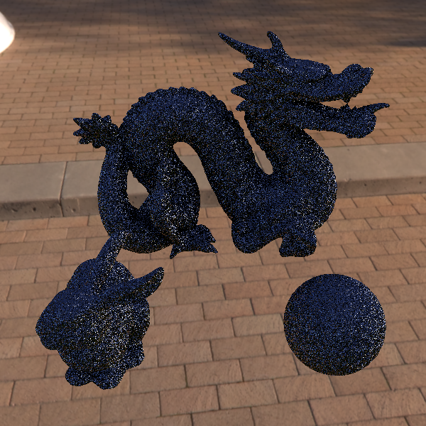
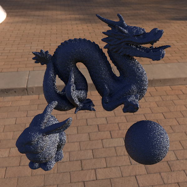
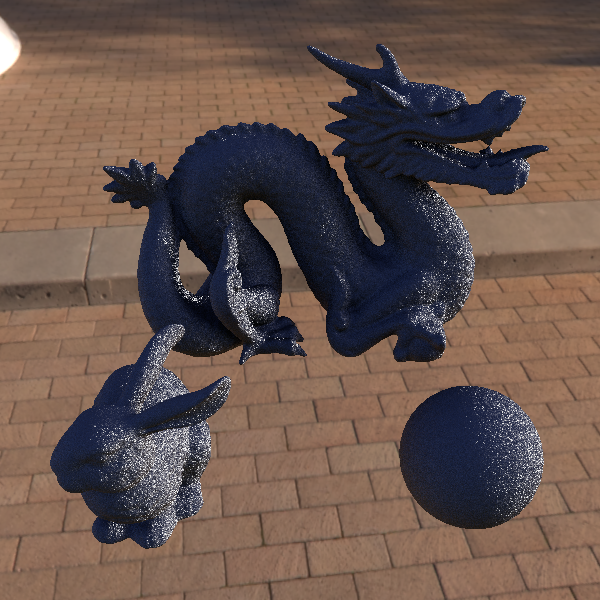
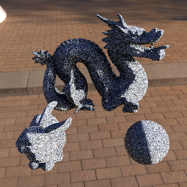
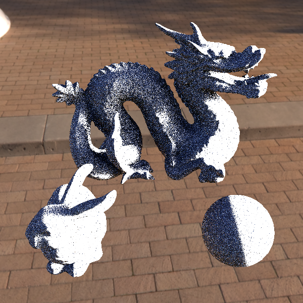
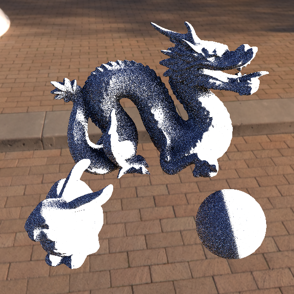
**Deferred Hybrid Path Tracing Series: Monte Carlo Integration and Next Event Estimation** ![Figure [fig:intro]: The Usual Suspects](intro.png border=1) It has been a while since the last article on my personal rendering project. In this post I'm going to talk about the current state of my GPU path tracer which now uses multiple importance sampling to approximate the light transport equation by combining BRDF sampling with light sampling. Furthermore, I'll show a how I've implemented mesh area lights and then list some of the improvements that I've made since last time. ## Basic Monte Carlo Integration and Importance Sampling Monte Carlo (MC) Integration is a method used to approximate an integral $\int_a^b F(x) dx$ by random sampling: $$ F_N = \frac{1}{N}\sum_{i=1}^{N}\frac{F(X_i)}{p(X_i)} $$ where $p(X_i)$ is the probability to sample $X_i$. I wont go over too much theory, the most important point to know is that MC integration gives us a framework to approximate the light transport equation by evaluating it at randomly sampled points. In the case we sample from a uniform distribution in the range $[0,1)$ we get: $$ F_N = \frac{1}{N}\sum_{i=1}^{N}F(X_i) $$ Sampling uniformly doesn't work well in most real-world scenes. This scenario is highlighted in the figure below where a uniform distribution would fail to sample the "interesting" areas of the function. This is where importance sampling comes in to help us. ![Figure [fig:uniform_fail]: Uniform Distribution Fail](placeholder.png border=1 width=85%) Importance sampling lets us modify our sampling strategy to better match the shape of the function we're integrating. As long as we correctly account for the sampling PDF the estimator will remain unbiased and converge towards the correct result. A commonly used importance sampling technique is cosine-weighted sampling. This sampling strategy favor samples that are oriented towards the surface's normal. It is what I currently use for BRDF sampling in my path tracer. I wont go into how we derive the normalization constant to make $cos\theta$ a valid PDF, but the normalization constant is $\frac{1}{\pi}$, giving us the PDF $p(w_i) = \frac{cos\theta}{\pi}$. My engine is currently limited to the Lambertian BRDF $f = \frac{\rho}{\pi}$, where $\rho$ is the albedo color. If we insert the BRDF into the light transport equation we get: $$ L_o(\textbf{x}, w_o) = \int_\Omega \frac{\rho}{\pi}L_i(w_i)(w_i \cdot \textbf{n})dw_i $$ where $\textbf{x}$ is the surface point and $(w_i \cdot \textbf{n})$ is the cosine term. We can rewrite the dot product as the cosine of the angle between the incoming light direction and the surface normal $(w_i \cdot \textbf{n}) = cos\theta_i$. Now you can see why cosine-weighted sampling is a good sampling strategy; it matches the shape of our integral! Rewriting the integral in terms of the estimator and inserting our PDF, it simplifies to: $$ F_N = \frac{1}{N}\sum_{i=1}^{N}\frac{ \frac{\rho}{\pi}L_i cos\theta_i}{\frac{cos\theta_i}{\pi}} = \frac{\rho}{N}\sum_{i=1}^{N} L_i $$ By rendering a sequence of images (showcasing every $32$ frames for a total of $96$ frames in the figure below) with this estimator using only the environment map, which is sampled when a path escapes the scene we get following:

Cosine-Weighted Sampling Frame 0

It looks pretty good especially in areas when the sun in the environment map isn't hit, with the caveat that the overall image brightness is dim. In areas where samples do hit the sun, we get a noisy result. This is because the PDF of our cosine-weighted sampling method doesn't match the radiance distribution of our environment map leading to poor convergence and high variance. If only we were able to add a specialized sampling strategy for the environment map to our estimator, that can work in tandem with cosine-weighted sampling without introducing bias... ## Next Event Estimation and Multiple Importance Sampling Next Event Estimation is a method where for every sample you split lighting into indirect (BRDF sampling) and direct light sampling contributions. In other words, you combine multiple sampling strategies in your estimator. As far as I know, there's no limitation on the types of light sources you sample, be it analytical lights such as point lights and directional lights, or lights where radiance distribution is spread over an area like mesh area lights and environment maps. As explained in the previous section, as long as we can correctly account for the sampling PDF we will be fine. However, we now have multiple sampling strategies, each with their own PDF. This means we need a combination strategy to combine them without introducing bias into the estimator. One such strategy is called the balance heuristic: $$ \hat{w_i}(x) = \frac{n_ip_i(x)}{\sum_k n_k p_k(x)} $$ where: * $\hat{w_i}$(x) is the weight for sampling method i * $n_i$ is the number of samples evaluated by the i'th sampling strategy * $p_i(x)$ is the probability to sample x for the i'th sampling strategy * The denominator is the sum of all PDFs over all strategies that could generate that sample In other words: the weight for one strategy is its PDF scaled by the number of samples taken, divided by the total contribution from all strategies that could have sampled that point. Inserting the balance heuristic into the Monte Carlo estimator gives us: $$ I = \sum_{i=1}^{N}\frac{1}{n_i}\sum_{j=1}^{N_i}w_i(X_{i,j})\frac{F(X_{i,j})}{p_i(X_{i,j})} $$ If we only take one sample per strategy (i.e., $n_i=1$, also known as single-sample multiple importance sampling), the estimator simplifies to: $$ I = \sum_{i=1}^{N}w_i(X_{i})\frac{F(X_{i})}{p_i(X_{i})} $$ Finally, to integrate this method into the renderer we need the PDF for every sampling strategy. We already have the PDF for cosine-weighted sampling, so lets improve our renderer by importance sampling the environment map:

Multiple Importance Sampling Frame 0

This sequence was taken every $4$ frames over $12$ frames in total, and as you can see its a clear improvement over using only BRDF sampling. The image is brighter and we've improved convergence in areas where the sun is visible. I wont go into the way I calculated the PDF for the environment map but if you're interested the method is described [here](https://www.pbr-book.org/3ed-2018/Monte_Carlo_Integration/2D_Sampling_with_Multidimensional_Transformations#Piecewise-Constant2DDistributions) in "Physically Based Rendering: From Theory To Implementation" by Matt Pharr et al. 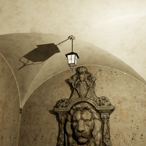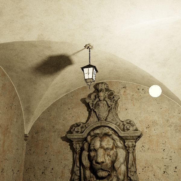## Mesh Area Lights I also added mesh area lights to my engine. This was done by constructing a discrete CDF over triangle areas. Let $A_{\Delta_i}$ be the area of triangle $i$ and $A = \sum_{i} A_{\Delta_i}$ the total mesh area. I select a triangle $i$ with probability: $$p(i) = \frac{A_{\Delta_i}}{A}$$ sampling uniformly within that triangle with PDF, $\frac{1}{A_{\Delta_i}}$, the overall PDF becomes: $$ p(x) = \frac{A_{\Delta_i}}{A} \cdot \frac{1}{A_{\Delta_i}} = \frac{1}{A} $$ To generate a sample, I pick a random number, $u$, in the range $[0,A)$, then perform a binary search on the CDF to find the corresponding triangle index. Once I have the triangle, I uniformly sample barycentrics to get a point on its surface and evaluate the lighting contribution from that point. If the scene contains multiple lights I sample one by a uniform distribution in the range $[0,N_l$), where $N_l$ is the total light count. The final PDF is then: $$ p(x) = \frac{1}{N_l \cdot A} $$ This scheme allows my renderer to produce visually realistic soft shadows with smooth and physically plausible penumbrae:

Small Spherical Light Source

## General Improvements Not an exhaustive list, but some of the more interesting things I've done: * Improved the shadow terminator based on this excellent [paper](https://www.yiningkarlli.com/projects/shadowterminator.html) by Matt Jen-Yuan Chiang, Yining Karl Li and Brent Burley * Sampling lights uniformly with a light list * Multithreaded asset loading (multiple producers/consumers) * Exposed command queues and fences in the RHI * Material editor * Cleaned up and nuked a lot of code in the RHI * Improved scene structure * Normal mapping * Reflective surfaces using Schlick's Fresnel approximation * World-space position from Z-buffer * ... ## Conclusion In this post we've covered some of the fundamentals of path tracing: monte carlo integration, importance sampling, multiple importance sampling and next event estimation. I've picked what I thought was most relevant to the write about in terms of theory and tried to keep it light. I still have tons of things I want to do with the project some of which I mentioned in the last post. For example, picking the right lights to sample from the light list... (restir wink wink nudge nudge...) However, the more theory I read, the more interested I get in internalizing the fundamentals of computer graphics, which I'm spending quite some time on at the moment. I've also been enrolled into an Industry Master of Science in Engineering degree, which I will be starting this autumn. The goal is to specialize in visual computing. This means that I'm also starting to think about some research projects I want to explore during my degree. All this to say that the coming articles will be focused more on theory as a way for me to internalize the fundamentals. I figure that I'm also going to do some short articles showcasing progress in material appearance modeling and interesting engine optimization efforts.